Question: A retaining wall is shown in Figure
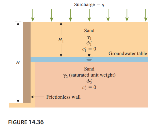
A retaining wall is shown in Figure 14.36. For each problem, determine the Rankine active force, Pa, per unit length of the wall and the location of the resultant.
> Determine the minimum factor of safety of a slope with the following parameters: H = 25 ft = 26.57°, ’ = 20° c’ = 300 lb/ft2 = 120 lb/ft3 ru = 0.5 Use Bishop and Morgenstern’s method.
> A loose, uncompacted sand fill 6 ft in depth has a relative density of 40%. Laboratory tests indicated that the minimum and maximum void ratios of the sand are 0.46 and 0.90, respectively. The specific gravity of solids of the sand is 2.65. What is the
> Referring to Figure 16.52 and using the ordinary method of slices, find the factor of safety with respect to sliding for the following trial cases.  = 45°, ’= 20°, câ
> Refer to Problem 16.19. Assume that the slope is subjected to earthquake forces. Let kh = 0.4 and kv = 0.5kh ((). Determine Fs using the procedure outlined in Section 16.11.
> Refer to Figure 16.51. Using Figure 16.24, find the factor of safety, Fs with respect to sliding for a slope with the following. Slope: 2.5H:1V = 16.5 kN/m3 ’ = 12° H = 12 ft c’ = 24 lb/ft2
> For the slope shown in Figure 16.48, find the height, H, for critical equilibrium. Given:  = 22°,  = 100 lb/ft3 , ’ = 15°, and c’ = 200 lb/f
> Refer to Figure 16.51. Using Figure 16.24, find the factor of safety, Fs with respect to sliding for a slope with the following. Slope: 1H:1V = 115 lb/ft3 ’ = 20° H = 30 ft c’ = 400 lb/ft2
> Refer to Figure 16.51. Using Figure 16.24, find the factor of safety, Fs with respect to sliding for a slope with the following. Slope: 2H:1V = 110 lb/ft3 ’ = 10° H = 50 ft c’ = 700 lb/ft2
> Refer to Figure 16.51. Use Figure 16.28 (’ > 0) to solve the following. If n’ = 2, ’ = 20°, c’ = 20 kN/m2 , and ï&se
> A clay slope is built over a layer of rock. Determine the factor of safety with kh = 0.4 for the slope with the following values. Height, H = 16 m Slope angle, = 30° Saturated unit weight of soil, sat = 17 kN/m3 Undrained shear strength, cu = 50 k
> A cut slope was excavated in a saturated clay. The slope angle, b, is equal to 40° with the horizontal. Slope failure occurred when the cut reached a depth of 8.5 m. Previous soil explorations showed that a rock layer was located at a depth of 12 m below
> Refer to Problem 16.13. What should the critical height of the slope be? What is the nature of the critical circle?
> The moisture content of a soil sample is 18.4%, and its dry unit weight is 100 lb/ft3 . Assuming that the specific gravity of solids is 2.65, Calculate the degree of saturation. What is the maximum dry unit weight to which this soil can be compacted wi
> Using the graph given in Figure 16.13, determine the height of a slope (1 vertical to 1 horizontal) in saturated clay with an undrained shear strength of 24 kN/m2 . The desired factor of safety against sliding is 2.5. Given: = 18 kN/m3 and D = 1.20.
> For the cut slope described in Problem 16.11, if we need a factor of safety of 2.0 against sliding, how deep should the cut be made?
> A cut slope is to be made in a saturated clay. Given: cu = 30 kN/m2 (f = 0 condition) and = 17 kN/m3 . The slope makes an angle b of 60° with the horizontal. Determine the maximum depth up to which the cut could be made. Assume that the critical surfac
> Refer to Figure 16.10. Using the soil parameters given in Problem 16.6, find the height of the slope, H, that will have a factor of safety of 2 against sliding. Assume that the critical surface for sliding is a plane.
> Refer to Figure 16.48. Given:  = 30°,  = 15.5 kN/m3 , ’ = 20°, and c’ = 15 kN/m2 . Find the height, H, which will have a factor of safety (F
> Redo Problem 15.8 when u = 10o and  = 0o.
> Refer to Figure 15.22. Given: u = 0,  = 0o, H = 5 m,  = 15 kN/m3 , ’ = 30o, and ’ = 15o. Estimate the passive force, Pp, per unit length of t
> Refer to the retaining wall shown in Figure 15.22. Given: u = 10o,  = 0,  = 19.2 kN/m3 , ’ = 35o, ’ = 21o, and H = 6 m. Estimate the passive
> Refer to Figure 15.22. Given: H = 5 m, = 0, = 0, = 18.7 kN/m3 , ’ = 30o, and ’ = 2/3 ’. Estimate the passive force, Pp, per unit length of the wall using the Kp values given by Shields and Tolunay’s (1973) method of slices (Table 15.1).
> Refer to the retaining wall in Problem 15.1. Estimate the passive force, Pp, per unit length of the wall using Sokolowskiı˘ (1965) solution by the method of characteristics (Table 15.3).
> For a given sandy soil, the maximum and minimum dry unit weights are 108 lb/ft3 and 92 lb/ft3 , respectively. Given Gs = 2.65, determine the moist unit weight of this soil when the relative density is 60% and the moisture content is 8%.
> Assume that the retaining wall shown in Figure 14.35 is frictionless. For each problem, determine the Rankine active force per unit length of the wall, the variation of active earth pressure with depth, and the location of the resultant.
> Refer to the retaining wall in Problem 15.1. Estimate the passive force, Pp, per unit length of the wall using Lancellotta’s (2002) analysis by the lower bound theorem of plasticity. Use Table 15.2.
> Refer to the retaining wall in Problem 15.1. Estimate the passive force, Pp, per unit length of the wall using Zhu and Qian’s (2000) method of triangular slices. Use Eq. (15.18).
> Refer to the retaining wall in Problem 15.1. Estimate the passive force, Pp, per unit length of the wall using Shields and Tolunay’s (1973) method of slices (Table 15.1).
> The cross section of a braced cut supporting a sheet pile installation in a clay soil is shown in Figure 15.25. Given: H = 12 m, clay = 17.9 kN/m3 ,  = 0, c = 75 kN/m2 , and the center-to-center spacing of struts in
> The elevation and plan of a bracing system for an open cut in sand are shown in Figure 15.24. Using Peck’s empirical pressure diagrams, determine the design strut loads. Given: sand = 18 kN/m3 , &ac
> A braced wall is shown in Figure 15.23. Given: H = 7 m, naH = 2.8 m, ’ = 30o, ’ = 20o,  = 18 kN/m3 , and c’ = 0. Determine the act
> Refer to the retaining wall described in Problem 15.8. If there is seepage in the backfill (as shown in Figure 15.8), what would be the magnitude of Pp based on the theory described in Section 15.7? Assume kx = kz and sat = 18 kN/m3 .
> Redo Problem 15.8 when ( = 0o and = 12o (Figure 15.7 and Table 15.6).
> A retaining wall has a vertical back face with a horizontal granular backfill. Given: H = 6 m, = 18.5 kN/m3 , ’ = 408, and ’ = 1/2’. Estimate the passive force, Pp, per unit length of the wall using Terzaghi and Peck’s (1967) wedge theory (Figure 15
> Refer to Section 14.13 and Figure 14.28. Determine the seismic earth pressure from the soil backfill on the retaining wall, considering = 110o, = 12o, ’ = 21o, ’ = 2/3 ’ = 14o, c’ = 30 kN/m2 , c’ a = 15 kN/m2 , H = 10 m, = 19 kN/m3 , q = 5 kN/m
> For a given sandy soil, emax = 0.75, emin = 0.46, and Gs = 2.68. What will be the moist unit weight of compaction (kN/m3) in the field if Dr = 78% and w = 9%?
> Refer to Section 14.13 and Figure 14.28. Determine the seismic earth pressure from the soil backfill on the retaining wall, considering = 105o, = 8o, ’ = 30o, ’ = 2/3 ’ = 20o, c’ = 0 kN/m2 , c’ a = 0 kN/m2 , H = 15 m, = 16.5 kN/m3 , q = 5 kN/m2
> Figure 14.10 provides a generalized case for the Rankine active pressure on a frictionless retaining wall with an inclined back and a sloping granular backfill. You are required to develop some compaction guidelines for the backfill soil when u = 10o and
> Refer to Figure 14.24. Given: H = 7.5 m, u = 10°, = 5°, = 17.9 kN/m3 , ’ = 28o, ’ = 1/2 ’, kh = 0.3, and kv = 0. Determine the active force, Pae, per unit length of the retaining wall. Also find the location of the resultant line of action of Pae.
> Consider the retaining wall shown in Figure 14.37. The height of the wall is 5 m, and the unit weight of the sand backfill is 18 kN/m3 . Using Coulomb’s equation, calculate the active force, Pa, on the wall for the following values of t
> Refer to the frictionless retaining wall shown in Figure 14.10. Given: H = 6 m, = 10°, u = 6°, ’ = 308, and ’ = 17 kN/m3 . Determine the magnitude, direction, and location of the active force Pa.
> Redo Problem 14.19, assuming that a surcharge pressure of 20 kN/m2 is applied on top of the backfill.
> An 8.5 m high retaining wall with a vertical back face retains a homogeneous, saturated soft clay. The saturated unit weight of the clay is 19.6 kN/m3 . Laboratory tests showed that the undrained shear strength, cu, of the clay is 22 kN/m2 . Make the ne
> For the data given in Problem 14.17, determine the Rankine passive force, Pp, per unit length of the wall, its location, and its direction.
> Figure 14.12 shows a frictionless wall with a sloping granular backfill. Given: H = 7 m, = 12°, ’ = 288, and = 18.6 kN/m3 . Determine the magnitude of active pressure, ’ , at the bottom of the wall. Determine the Rankine active force, Pa, per u
> For the partially submerged backfill in Problem 14.13 (Figure 14.36), determine the Rankine passive force per unit length of the wall and the location of the resultant.
> For a given sand, the maximum and minimum void ratios are 0.78 and 0.43, respectively. Given Gs = 2.67, determine the dry unit weight of the soil in kN/m3 when the relative density is 65%.
> A retaining wall is shown in Figure 14.36. For each problem, determine the Rankine active force, Pa, per unit length of the wall and the location of the resultant.
> A retaining wall is shown in Figure 14.36. For each problem, determine the Rankine active force, Pa, per unit length of the wall and the location of the resultant.
> Consider the clay specimen in Problem 13.8. A consolidated-undrained triaxial test was conducted on the same clay with a chamber pressure of 15 lb/in2 . The pore pressure at failure is (ud)f = 4.8 lb/in2 . What would be the major principal effective str
> In a consolidated-drained triaxial test on a clay, the specimen failed at a deviator stress of 18 lb/in2 . If the effective stress friction angle is known to be 31°, what was the effective confining pressure at failure?
> For a normally consolidated clay specimen, the results of a drained triaxial test are as follows. Chamber-confining pressure = 125 kN/m2 Deviator stress at failure = 175 kN/m2 Determine the soil friction angle ’.
> The relationship between the relative density, Dr, and the angle of friction, ’, of a sand can be given as ’ 5 28 1 0.18 Dr (Dr in %). A drained triaxial test was conducted on the same sand with a chamber-confining pressure of 150 kN/m2 . Calculate the
> Refer to Figure 13.62. Shear strength parameters are needed for the design of a foundation placed at a depth of 2 m in the silty sand layer. Soils collected from this sand were compacted in the direct shear mold (diameter 5 63.5 mm) at the same dry unit
> During a subsoil exploration program, undisturbed normally consolidated silty clay samples were collected in Shelby tubes from location A as shown in Figure 13.62. Following are the results of four drained, direct shear tests conducted on the clay samp
> For a dry sand specimen in a direct shear test box, the following are given. Size of specimen: 2.5 in. ×2.5 in. × 1.25 in. (height) Angle of friction: 33° Normal stress: 28 lb/in2 Determine the shear force required to cause failure.
> Refer to Problem 3.18. Given that the borrow pit has a moisture content of 11% and Gs = 2.7, determine: Moist unit weight of the borrow soil Degree of saturation of the borrow soil Moist unit weight of the compacted backfill
> Refer to the clay soil in Figure 13.63. If the natural moisture content is 28%, estimate the undrained shear strength of remolded clay using the relationships given in Table 13.5 by Leroueil et al. (1983) Terzaghi et al. (1996)
> A 15 m thick normally consolidated clay layer is shown in Figure 13.63. The liquid limit and plastic limit of the soil are 39 and 20, respectively. Using Eq. (13.53) given by Skempton (1957), estimate the undrained cohesion at a depth of 11 m below the
> Consider the specimen in Problem 13.1b. What are the principal stresses at failure? What is the inclination of the major principal plane with the horizontal?
> Results of two consolidated-drained triaxial tests on a clayey soil are as follows. Using the failure envelope given in Example 13.18 (q’ =  1 p’ tan ), determine the following (do
> Undisturbed samples from a normally consolidated clay layer were collected during a field exploration program. Drained triaxial tests showed that the effective friction angle at ’ = 28°. The unconfined compressive strength, u, of a similar specimen was
> A consolidated-undrained triaxial test was conducted on a dense sand with a chamber-confining pressure of 20 lb/in2 . Results showed that ’ = 24° and = 31°. Determine the deviator stress and the pore water pressure at failure. If the sand were loose,
> If a consolidated-drained test is conducted on the clay specimen of Problem 13.15 with the same chamberconfining pressure of 150 kN/m2 , what would be the deviator stress at failure?
> The shear strength of a normally consolidated clay can be given by the equation f = ’ tan 27°. Following are the results of a consolidated-undrained test on the clay. Chamber-confining pressure = 150 kN/m2 Deviator stress at failure = 120 kN/m2 Deter
> A clay sample was consolidated in a triaxial test chamber under an all-around confining pressure of 22 lb/in2 . The sample was then loaded to failure in an undrained condition by applying an additional axial stress of 28 lb/in2 . A pore water pressure se
> Consider the triaxial tests in Problem 13.12. What are the normal and shear stresses on a plane inclined at 40° to the major principal plane for Specimen I? What are the normal and shear stresses on the failure plane at failure for Specimen II?
> Refer to Figure 3.13. After the construction of a concrete retaining wall, backfill material from a nearby borrow pit was brought into the excavation behind the wall and compacted to a final void ratio of 0.8. Given that the soil in the borrow pit has a
> The results of two consolidated-drained triaxial tests on a clay are given here. Calculate the shear strength parameters of the soil.
> A consolidated-drained triaxial test was conducted on a normally consolidated clay with a chamber pressure, 3 = 25 lb/in2 . The deviator stress at failure is (ud)f = 33 lb/in2 . Determine the following. The angle of friction ’ The angle u that the f
> Following are the results of consolidated-undrained triaxial tests on undisturbed soils retrieved from a 4 m thick saturated clay layer in the field (sat = 19 kN/m3 ). Estimate graphically the Mohr–Coulomb shear stren
> The following data are given for a direct shear test conducted on dry silty sand: Specimen dimensions: 63 mm × 63 mm × 25 mm (height) Normal stress: 105 kN/m2 Shear force at failure: 300 N Determine the angle of friction, ’. For a normal stress of 18
> The laboratory consolidation data for an undisturbed clay specimen are as follows. e1 = 1.1 ’ 1 = 1 ton/ft2 e2 = 0.9 ’ 2 = 3 ton/ft2 What is the void ratio for a pressure of 3.5 ton/ft2 ? (Note: ’ c = 0.8 ton/ft2 .)
> The coordinates of two points on a virgin compression curve are as follows. e1 = 0.82 ’ 1 = 2500 lb/ft2 e2 = 0.70 ’2 = 4000 lb/ft2 Determine the void ratio that corresponds to a pressure of 6000 lb/ft2 .
> Refer to Figure 12.42. Given: H1 = 5 ft, H2 = 7 ft, H3 = 6 ft, and Ds = 3000 lb/ft2 . Also, Clay: e = 1.1, Gs = 2.72, LL = 45 Sand: e = 0.58, Gs = 2.65 Estimate the primary consolidation settlement if the pre-consolidation pressure is 3500 lb/ft2 .Ass
> Refer to Figure 12.42. Given: H1 = 2.5 m, H2 = 2.5 m, H3 = 3 m, and  = 100 kN/m2 . Also, Sand: e = 0.64, Gs = 2.65 Clay: e = 0.9, Gs = 2.75, LL = 55 Estimate the primary consolidation settlement of the
> Figure 12.42 shows a soil profile. The uniformly distributed load on the ground surface is Ds. Given:  = 1000 lb/ft2 , H1 = 8 ft, H2 = 15 ft, and H3 = 17 ft. Also, Sand: dry = 110 lb/ft3 , ï
> The results of a laboratory consolidation test on a clay specimen are the following. Given the initial height of specimen 5 0.748 in., Gs = 2.68, mass of dry specimen = 95.2 g, and area of specimen = 4.91 in2: Plot the e-log â&
> Refer to Problem 3.16. Determine the weight of water, in lb, that will be in 2.5 ft3 of the soil when saturated.
> Repeat Problem 12.2 using the following values
> Foundation engineers are often challenged by the existence of soft compressible soils at the construction site. Figure 12.44 shows a soil profile with a silty sand ( = 17 kN/m3 ; sat = 19.2 kN/m3 ) underlain by high pl
> The following are the results of a consolidation test. Plot the e-log ’ curve. Using Casagrande’s method, determine the preconsolidation pressure. Calculate the compression index, Cc, from the lab
> Refer to Figure 12.43. Given that B = 1 m, L = 3 m, and Q = 110 kN, calculate the primary consolidation settlement of the foundation.
> A normally consolidated clay layer is 3 m thick (one-way drainage). From the application of a given pressure, the total anticipated primary consolidation settlement will be 80 mm. What is the average degree of consolidation for the clay layer when the se
> A 3 m thick layer of saturated clay (two-way drainage) under a surcharge loading underwent 90% primary consolidation in 100 days. The laboratory test’s specimen will have two-way drainage. Find the coefficient of consolidation of clay for the pressure r
> The time for 50% consolidation of a 25 mm thick clay layer (drained at top and bottom) in the laboratory is 225 s. How long (in days) will it take for a 2 m thick layer of the same clay in the field (under the same pressure increment) to reach 50% consol
> For a laboratory consolidation test on a clay specimen (drained on both sides), the following were obtained. Thickness of the clay layer = 25 mm ’ 1 = 200 kN/m2 e1 = 0.73 ’ 2 = 400 kN/m2 e2 = 0.61 Time for 50% consolidation (t50) = 2.8 min Determi
> For a normally consolidated clay, the following are given. ’ o = 2 ton/ft2 e = eo = 1.21 ’ o + ’ = 4 ton/ft2 e = 0.96 The hydraulic conductivity k of the clay for the preceding loading range is 1.8 3 1024 ft/day. How long (in days) will it ta
> The time for 50% consolidation of a 1 in. thick clay layer (drained at top and bottom) in the laboratory is 2 min, 20 s. How long (in days) will it take for an 8 ft thick layer of the same clay in the field (under the same pressure increment) to reach 30
> The moist unit weights and degrees of saturation of a soil are given in the table. Determine: e Gs
> The coordinates of two points on a virgin compression curve are as follows. e1 = 1.7 ’ 1 = 150 kN/m2 e2 = 1.48 ’ 2 = 400 kN/m2 Determine the coefficient of volume compressibility for the pressure range stated. Given that cv = 0.002 cm2 /s, dete
> Following are the relationships of e and ’for a clay soil. For this clay soil in the field, the following values are given: H = 4.5 ft, ’ o = 0.7 ton/ft2 , and &a
> Refer to Problem 12.6. Given: cv = 2.8 × 10– 6 m2 /min. How long will it take for 60% consolidation to occur?
> Following are the results of a laboratory consolidation test on a sample of undisturbed clay obtained from the field The height of the specimen at the beginning of the test was 1.9 cm, and the diameter was 6.35 cm. The mass of the dry specimen was 91 g
> A shallow foundation supported by a silty sand is shown in Figure 11.6. Given: Length: L = 3 m Width: B = 3 m Depth of foundation: Df = 1.5 m Thickness of foundation: t = 0.25 m Load per unit area: = 150 kN/m2 Ef = 15 3 106 kN/m2 The silty sand has t
> A rigid, reinforced concrete foundation is subjected to a column load of 87,000 lb. The foundation plan measures 8 ft × 8 ft and rests on 21 ft (5 H’) of layered soil underlain by rock. The soil layers have the following ch
> A vertical column load, P = 600 kN, is applied to a rigid concrete foundation with dimensions B = 1 m and L = 2 m, as shown in Figure 11.11. The foundation rests at a depth Df = 0.75 m on a uniform dense sand with the following properties. Average modulu
> Repeat Problem 10.8 with the following data. q1 = 300 kN/m x1 = 4 m q2 = 260 kN/m x2 = 3 m z = 3 m
> Refer to Figure 10.50. Determine the vertical stress increase, s, at point A with the following values. q1 = 75 kN/m x1 = 2 m q2 = 300 kN/m x2 = 3 m z = 2 m
> Point loads of magnitude 8.9, 17.8, and 26.7 kN act at A, B, and C, respectively (Figure 10.49). Determine the increase in vertical stress at a depth of 3 m below point D. Use Boussinesq’s equation.

