Question: Imagine sampling a population of plants or
Imagine sampling a population of plants or animals to determine the distribution of individuals across the habitat. One of the most basic questions that you could ask is, “How are individuals in the population distributed across the study area?†How might they be distributed? The three basic patterns that we’ve discussed in this section are clumped, random, and regular distributions. The first step toward testing statistically between these three types of distributions is to sample the population to estimate the mean (p. 18) and variance (pp. 88–89) in density of the population across the study area. The theoretical relationships between variance in density and mean density in clumped, random, and regular distributions are as follows:
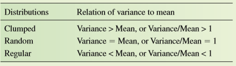
How do we connect these relationships between variance and mean density with what we see on the ground? In a clumped distribution, many sample plots will contain few or no individuals while some will contain a large number. As a consequence, the variance among sample plots will be high and the variance in density will be greater than the mean. In contrast, sample plots of a population with a regular distribution will all include a similar number of individuals. As a result, the variance in density across samples will be low when taken from a population with a regular distribution; therefore, the variance will be less than the mean. Meanwhile, in a randomly distributed population, the variance in density across the habitat will be approximately equal to the mean density.
Consider the following samples of three different populations of herbaceous plants growing on a desert landscape. Each sample is the number counted in a randomly located 1Â m2 area at the study site.
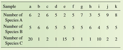
The distribution of individuals among the samples of species A, B, and C is quite different. For instance, each of the samples contained approximately the same number of individuals of species B. In contrast, the numbers of species C varied widely among samples. Meanwhile, counts of species A showed a level of variation somewhere in between variations in species B and C. The samples of species A, B, and C may give the impression of random, regular, and clumped distributions. We can quantify our visual impressions by calculating the sample means and sample variances for the densities of species A, B, and C:
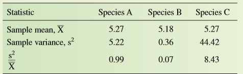
While the mean density calculated from the samples was very similar for all three species, their variance in density among samples was quite different. As a consequence, the ratios of sample variance to sample means, /were also different. While/for species A was nearly 1, this ratio was much less than 1 for species B, and much greater than 1 for species C. These results show how the /ratios we calculated that species A has a random distribution, that species B has a regular distribution, and that C has a clumped distribution? While it is likely that they do, in science we need to attach probabilities to such conclusions. To do that, we need to consider these samples of species A, B, and C from a statistical perspective. We will look at the statistics of these samples in chapter 10 (see p. 236).
Required:
1. According to the results of Phillips and MacMahon, what is the approximate value of the ratio of variance in shrub density to mean shrub density (variance/mean) for young, medium-age, and older creosote bushes (see fig. 9.13)?
Figure 9.13:

Transcribed Image Text:
Distributions Relation of variance to mean Clumped Variance > Mean, or Variance/Mean > 1 Random Variance = Mean, or Variance/Mean = 1 %3D Regular Variance < Mean, or Variance/Mean < 1 Sample а b c d f ghi j k e Number of 6 2 6 5 2 5 7 3 5 9 8 Species A Number of Species B 5 6 6 5 5 5 5 6 4 5 5 Number of 20 1 2 1 15 3 1 1 10 2 Species C 2. Statistic Species A Species B Species C Sample Mean, X Sample variance, s² 5.27 5.18 5.27 5.22 0.36 44.42 0.99 0.07 8.43 X .2
> From a life table and a fecundity schedule, you can estimate the geometric rate of increase, l, the average reproductive rate, R0 , the generation time, T, and the per capita rate of increase, r. That is a lot of information about a population. What mini
> What values of R0 indicate that a population is growing, stable, or declining? What values of r indicate a growing, stable, or declining population?
> Concept 10.5 says that we can use the information in life tables and fecundity schedules to estimate some characteristics of populations (R0, T, r). Why does Concept 10.5 use the word “estimate” rather than “calculate”? In putting together your answer, t
> Draw hypothetical age structures for growing, declining, and stable populations. Explain how the age structure of a population with highly episodic reproduction might be misinterpreted as indicating population decline. How might population ecologists avo
> Population ecologists have assumed that populations of species with very high reproductive rates, those with offspring sometimes numbering in the millions per female, must have a type III survivorship curve even though very few survivorship data exist fo
> Ecologists predict that global diversity is threatened by land use change and by the reductions in habitat area and the fragmentation that accompany land use change. Vitousek (1994) suggested that land use change may be the greatest current threat to bio
> Of the three survivorship curves, type III has been the least documented by empirical data. Why is that? What makes this pattern of survivorship difficult to study?
> Compare cohort and static life tables. What are the main assumptions of each? In what situations or for what organisms would it be practical to use either?
> Outline Müller’s (1954, 1974) colonization cycle. If you were studying the colonization cycle of the freshwater snail Neritina latissima, how would you follow colonization waves upstream? How would you verify that these colonization waves gain individual
> Can the analyses by Damuth (1981) and by Peters and Wassenberg (1983) be combined with that of Rabinowitz (1981) to make predictions about the relationship of animal size to its relative rarity? What two attributes of rarity, as defined by Rabinowitz, ar
> Outline Rabinowitz’s classification (1981) of rarity, which she based on size of geographic range, breadth of habitat tolerance, and population size. In her scheme, which combination of attributes makes a species least vulnerable to extinction? Which com
> Use the empirical relationship between size and population density observed in the studies by Damuth (1981) (see fig. 9.19) and Peters and Wassenberg (1983) (see fig. 9.20) to answer the following: For a given body size, which ge
> Suppose that in the near future, the fish crow population in North America declines because of habitat destruction. Now that you have reviewed the large-scale distribution and abundance of the fish crow (see fig. 9.15 b), devise a conservatio
> Suppose one plant reproduces almost entirely from seeds, and that its seeds are dispersed by wind, and a second plant reproduces asexually, mainly by budding from runners. How should these two different reproductive modes affect local patterns of distrib
> How might the structure of the environment; for example, the distributions of different soil types and soil moisture, affect the patterns of distribution in plant populations? How should interactions among plants affect their distributions?
> What kinds of interactions within an animal population lead to clumped distributions? What kinds of interactions foster a regular distribution? What kinds of interactions would you expect to find within an animal population distributed in a random patter
> As we saw in chapters 18 and 19, nitrogen availability seems to control the rates of several ecosystem processes. How should nitrogen enrichment affect rates of primary production and decomposition in terrestrial, freshwater, and marine environments? How
> Spruce trees, members of the genus Picea, occur throughout the boreal forest and on mountains farther south. For example, spruce grow in the Rocky Mountains south from the heart of boreal forest all the way to the deserts of the southern United States an
> What confines Encelia farinosa to upland slopes in the Mojave Desert? Why is it uncommon along desert washes, where it would have access to much more water? What may allow E. frutescens to persist along desert washes whereas E. farinosa cannot?
> The oceans cover about 360 million km 2 and have an average depth of about 4,000 m. What proportion of this aquatic system receives sufficient light to support photosynthesis? Make the liberal assumption that the photic zone extends to a depth of 200 m.
> Behavioral ecologists have argued that naked mole rats are eusocial. What are the major characteristics of eusociality and which of those characteristics are shared by naked mole rats?
> The details of experimental design are critical for determining the success or failure of both field and laboratory experiments. Results often depend on some small details. For instance, why did Jennifer Jarvis wait 1 year after establishing her laborato
> The results of numerous studies indicate nonrandom mating among plants at least under some conditions. These results lead to questions concerning the biological mechanisms that produce these nonrandom matings. How might the maternal plant control or at l
> Discuss the scorpionfly mating system. Pay particular attention to the potential roles of intersexual and intrasexual selection in scorpionflies.
> Endler set up two experiments, one in the greenhouse and one in the field. What were the advantages of the greenhouse experiments? What were the shortcomings of the greenhouse experiments? Endler also set up field experiments along the Aripo River. What
> Endler (1980) pointed out that though field observations are consistent with the hypothesis that predators may exert natural selection on guppy coloration, some other factors in the environment could be affecting variation in male color patterns among gu
> One of the basic assumptions of the material presented in chapter 8 is that the form of reproduction will exert substantial influence on social interactions within a species. How might interactions differ in populations that reproduce asexually versus on
> In chapter 23, we briefly discussed how humans have more than doubled the quantity of fixed nitrogen cycling through the biosphere. In chapter 15, we reviewed studies by Nancy Johnson (1993) on the effects of fertilization on the mutualistic relationship
> The introduction to chapter 8 included sketches of the behavior and social systems of several fish species. Using the concepts that you have learned in this chapter, revisit those examples and predict the forms of sexual selection occurring in each speci
> The data of Iriarte and colleagues (1990) suggest that prey size may favor a particular body size among pumas (see fig. 7.19). However, this variation in body size also correlates well with latitude; the larger pumas live at high latitudes. C
> The rivers of central Portugal have been invaded, and densely populated by the Louisiana crayfish Procambarus clarki, which looks like a freshwater lobster about 12 to 14 cm long. The otters of these rivers, which were studied by Graça and F
> What kinds of animals would you expect to have type 1, 2, or 3 functional responses? How should natural selection for better prey defense affect the height of functional response curves? How should natural selection for more effective predators affect th
> Ecologists explore the relationships between organisms and environment using the methods of science. The series of boxes called “Investigating the Evidence” that are found throughout the chapters of this book discuss v
> One of the most common and important steps in the processing of data is the production of summary statistics. First, what is a statistic? A statistic is a number that is used by scientists to estimate a measurable characteristic of an entire population.
> In chapter 2 (p. 18) we determined the sample mean. However, while the sample mean is one of the most common and useful of summary statistics, it is not the most appropriate statistic for some situations. One of the assumptions underlying the use of the
> In chapter 6 (see p. 136) we considered the number of samples necessary to obtain a reasonably precise estimate of the number of species in two simple communities. In chapter 16 (see p. 359) we reconsidered the same question in relation to very complex c
> Suppose you are studying the exchange of organic matter between forests and streams and the landscape you are studying is a mosaic of patches of two forest types: deciduous and coniferous. Part of your study involves determining whether there is a differ
> The question we consider now is how to represent variation in samples drawn from populations in which measurements or observations do not have normal distributions. When analyzing normally distributed measurements, depending on our purpose, we can estima
> In chapter 18 (p. 406) we compared samples from two populations using the t- test to judge whether there was a statistically significant difference between the populations. While the t -test is one of the most valuable tools for comparisons of pairs of s
> I n chapter 17, we used confidence intervals to compare the biomasses of two populations of the diatom-feeding caddisfly, Neothremma alicia. That comparison indicated that the population living in a stream that had flooded recently had a lower biomass p
> Design a planetary ecosystem based entirely on chemosynthesis. You might choose an undiscovered planet of some distant star or one of the planets in our own solar system, either today or at some distant time in the past or future.
> In chapter 15 we reviewed how to calculate confidence intervals for the true population mean as: Here, we will use the confidence intervals calculated from samples of two populations to create a visual comparison of the populations. Suppose you are st
> How many species are there? This is one of the most fundamental questions that an ecologist can ask about a community. With increasing threats to biological diversity, species richness is also one of the most important community attributes we might measu
> n chapter 14 we reviewed how to calculate the standard error, s _ X, which is an estimate of variation among means of samples drawn from a population. Here, we will use the standard error to calculate a confidence interval. A confidence interval is a ran
> When we introduced the sample mean, we pointed out how it is an estimate of the actual, or true, population mean. A second sample from a population would probably have a different sample mean and a third sample would have yet another. How close is a give
> Field experiments have played a key role in the assessment of the importance of competitive interactions in nature. Joseph Connell (1974) and Nelson Hairston, Sr. (1989), two of the pioneers in the use of field experiments in ecology, outlined their prop
> Suppose you are studying the life history of three species of herbaceous plants in a desert landscape. As part of that study, you are interested in determining the pattern of distribution of individuals in each population. Your hypothesis states that the
> Ecologists often ask questions about observed frequencies of individuals in a population relative to some theoretical or expected frequencies. For example, an ecologist studying the nesting habits of Darwin’s finches may be interested i
> In chapter 1, we reviewed the roles of questions and hypotheses in the process of science. Briefly, we considered how scientists use information to formulate questions about the natural world and convert their questions to hypotheses. A hypothesis, we sa
> As we have seen, the extent to which phenotypic variation in a trait is determined by genetic variation affects its potential to evolve by natural selection. In other words, the potential for a trait to evolve is affected by the trait’s
> What advantage does advertising give to noxious prey? How would convergence in aposematic coloration among several species of Müllerian mimics contribute to the fitness of individuals in each species? In the case of Batesian mimicry, what are the costs a
> Ecologists are often interested in the relationship between two variables, which we might call X and Y. For example, in chapter 7 we reviewed a study of how the size of pumas, variable X, is related to the size of prey that they take, variable Y (see fig
> The number of observations included in a sample, that is, sample size, has an important influence on the level of confidence we place on conclusions based on that sample. Let’s examine a simple example of how sample size affects our est
> One of the most powerful ways to test a hypothesis is through an experiment. Experiments used by ecologists generally fall into one of two categories—field experiments and laboratory experiments. Field and laboratory experiments generally provide complem
> In chapter 2 we calculated the sample mean and in chapter 3 we determined the sample median. The mean and median are different ways of representing the middle, or typical, within a sample of a population. Another important question we can ask is, how muc
> Throughout this series of discussions of investigating the evidence, we have emphasized one main source of evidence— original research. While original research is the foundation on which science rests, our emphasis has neglected one of
> What conclusion can we draw from the parallel between photosynthetic response curves in plants and functional response curves of animals?
> Why are plants such as mosses living in the understory of a dense forest, which show higher rates of photosynthesis at low irradiance, unable to live in environments where they are exposed to full sun for long periods of time?
> In type 3 functional response, what mechanisms may be responsible for low rates of food intake—compared to type 1 and type 2 functional response—at low food densities?
> Why are all the endothermic fish relatively large?
> Can behavioral thermoregulation be precise? What evidence supports your answer?
> What are the relative advantages and disadvantages of being an herbivore, a detritivore, or a carnivore? What kinds of organisms were left out of our discussions of herbivores, detritivores, and carnivores? Where do parasites fit? Where does Homo sapiens
> Why would it be a disadvantage for Encelia farinose (p. 110) to produce highly reflective, pubescent leaves in both hot and cool seasons?
> There is genetic evidence that mating between G. magnirostris and G. fortis (see fig. 13.8) may have helped establish sufficient genetic variation in the population of G. fortis at El Garrapatero for the distribution of beak sizes at that site (see fig.
> Why is rapid, human-induced environmental change a threat to natural populations?
> Why may the history of CFCs in the atmosphere in the years following the Montreal Protocol offer encouragement as humanity strives to reverse the modern buildup of atmospheric CO 2?
> Are there uncertainties remaining regarding global warming?
> What aspects of global warming are widely supported by available evidence?
> What can we conclude from the evidence summarized by figures 23.20 to 23.23? Figures 23.20: Figures 23.23: Continue to next pages………. The concentration of "C in the atm
> What component of species diversity (see chapter 16, p. 360) did Tilman’s research group manipulate in their studies? What other components of species diversity could influence rates of primary production? Continue to next pages
> How can we explain the results of Lubchenco’s manipulation of Littorina populations summarized in figure 17.8? Figure 17.8:
> What was the major limitation of Paine’s first removal experiment involving Pisaster?
> In chapter 7, we emphasized how the C 4 photosynthetic pathway saves water, but some researchers suggest that the greatest advantage of C 4 over C 3 plants occurs when CO2 concentrations are low. What is the advantage of the C 4 pathway when CO2 concentr
> Paine discovered that intertidal invertebrate communities of higher diversity include a higher proportion of predator species. Did this pattern confirm Paine’s predation hypothesis?
> Why is rapid, human-induced environmental change a threat to natural populations?
> Suppose you discover that the fish species inhabiting small, isolated patches of coral reef use different vertical zones on the reef face—some species live down near the sand, some live a bit higher on the reef, and some higher still. Based on this patte
> Can we link increased nutrient availability during the Park Grass Experiment with decreased environmental complexity?
> Does Tilman’s finding that Asterionella and Cyclotella exclude each other under certain conditions but coexist under other conditions violate the competitive e xclusion principle (see chapter 13, p. 286)?
> Both mathematical and laboratory models offer valuable insights into the dynamics of predator-prey systems. What are some advantages and limitations of each approach?
> According to Keller’s theory, under what general conditions would the mutant Helianthella quinquenervis, lacking extrafloral nectaries, increase in frequency in a population and displace the typical plants that produce extrafloral nectaries?
> Suppose you discover a mutant form of Helianthella quinquenervis that does not produce extrafloral nectaries. What does Keller’s theory predict concerning the relative fitness of these mutant plants and the typical ones that produce extrafloral nectaries
> Why is it not surprising that snowshoe hare populations are controlled by a combination of factors, food and predators (see fig. 14.15), and not by a single environmental factor? Figure 14.15:
> When the coupled cycling of lynx and snowshoe hare populations (see fig. 14.14) was first described, many concluded that lynx control snowshoe hare populations. Why are lynx not the primary factor controlling snowshoe hare populations even th
> In what kinds of environments would you expect to find the greatest predominance of C 3 , C 4 , or CAM plants? How can you explain the co-occurrence of two, or even all three, of these types of plants in one area?
> Is there any way that predators could alter the outcome of competition as shown in figure 13.14 a, where species 1 excludes species 2, and in figure 13.14 b, where species 2 excludes species 1? Figure 13.14:
> Can we conclude that interspecific competition commonly restricts species to realized niches in nature, based on the results of mathematical models and laboratory experiments?
> Paramecium aurelia and P. caudatum coexisted for a long period when fed full-strength food compared to when they were fed half that amount. What does this contrast in the time to competitive exclusion suggest about the role of food supply on competition
> Why might medium ground finch population responses to short-term, episodic increases in rainfall (see fig. 11.17) differ from their responses to increases in rainfall lasting for years or decades? Figure 11.17:
> Where would you place the following plant species, in Grime’s and in Winemiller and Rose’s classifications of life histories (see figs. 12.20 and 12.21)? The plant species lives in an environment where it has access to
> If a concept, such as r and K selection, does not fully represent the richness of life history variation among species, can it still be valuable to science?
> What appears to set the carrying capacity for medium ground finches on Daphne Major Island?
> Why can we be sure that all animal and plant populations are under some form of environmental control?
> How would human mortality patterns have to change for our species to shift from type I to type II survivorship?
> Female cottonwood trees (Populus species) produce millions of seeds each year. Does this information give you a sound basis for predicting their survivorship pattern?
> Why don’t plants use highly energetic ultraviolet light for photosynthesis? Would it be impossible to evolve a photosynthetic system that uses ultraviolet light? Does the fact that many insects see ultraviolet light change your mind? Would it be possible
> Review evidence that the El Niño Southern Oscillation significantly influences populations around the globe. Much of our discussion in chapter 23 focused on the effects of the El Niño Southern Oscillation on populations. Considering our discussions in ch
> How would substantial emigration and immigration affect estimates of survivorship within a population, where estimates are based on age distributions?
> What does the position of pines along moisture gradients in both the Santa Catalina Mountains of Arizona (see fig. 9.17) and the Great Smoky Mountains of Tennessee (see fig. 9.18) suggest about pine water relations? FigureÂ
> Why might the winter aggregations of crows occur mainly along river valleys?
> What factors might be responsible for the aggregation of American crows in winter (see fig. 9.15)? Figure 9.15: High The American crow, which is very widely distributed, is most abundant in a limited number of "hot spots." Low (a) Withi

